#DualGraphs

2022-12-18

#LogicalGraphs • 16
oeis.org/w/index.php?title=Log

#Duality • Logical and Topological
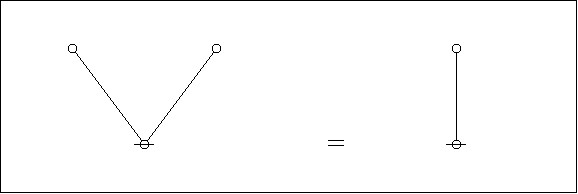
Turning to the #InitialEquation or #LogicalAxiom whose text expression is \(``\texttt{(}~\texttt{)(}~\texttt{)}=\texttt{(}~\texttt{)}",\) Figure 8 shows the planar maps and their corresponding #DualGraphs superimposed.

Figure 8
oeis.org/w/images/0/09/Logical

#Logic #Peirce #SpencerBrown #LawsOfForm
#PropositionalCalculus #BooleanFunctions
#GraphTheory #ModelTheory #ProofTheory

Figure 8 is a composite picture for the Formal Equation in Figure 1.  It illustrates the mapping of alpha graphs to dual graphs by overlaying the alpha graphs in Figure 1 with their corresponding dual graphs.

We may think of the picture as composed of two layers.

Layer 1 shows the alpha graphs for the First Initial Equation, previously shown in Figure 1 and again in Figure 7.  Proceeding from left to right in Layer 1, there is a form on the left hand side, an equal sign, and a form on the right hand side.

The form on the left consists of two circles drawn next to each other a space apart.

The form on the right consists of a single circle.

Layer 2 shows the dual graphs corresponding to the alpha graphs in Layer 1.  Proceeding from left to right in Layer 2, there is a form on the left hand side, an equal sign, and a form on the right hand side.

The form on the left is a graph-theoretic rooted tree, in this case consisting of two edges sharing a common root.  The root is placed outside and below the two circles.  The first edge extends to the interior of the circle on the left, where it meets its terminal node.  The second edge extends to the interior of the circle on the right, where it meets its terminal node.

The form on the right consists of a single rooted edge, or a rooted path of length one.  It extends from its root outside the single circle to its terminal node inside the circle.
2022-12-10

#LogicalGraphs • 10
oeis.org/w/index.php?title=Log

Figure 4 illustrates the mapping of #AlphaGraphs to #DualGraphs by overlaying the alpha graphs of Figure 2 with their corresponding dual graphs.

Figure 4. Alpha Graphs and Dual Graphs for the Second #InitialEquation
oeis.org/w/images/3/3f/Logical

It is usual to think of ourselves as observing alpha graphs from the outermost region of the plane and we mark that by mapping that region to a node singled out as the “root” of the dual.

#Logic #Peirce

Figure 4 is a composite picture for the Formal Equation in Figure 2. It illustrates the mapping of alpha graphs to dual graphs by overlaying the alpha graphs in Figure 2 with their corresponding dual graphs.

We may think of the picture as composed of two layers.

Layer 1 shows the alpha graphs for the Second Initial Equation, previously shown in Figure 2 and again in Figure 3.  Proceeding from left to right in Layer 1, there is a form on the left hand side, an equal sign, and a form on the right hand side.

The form on the left hand side consists of two concentric circles.

The form on the right hand side is shown as white space or a blank area.

Layer 2 shows the dual graphs corresponding to the alpha graphs in Layer 1. Proceeding from left to right in Layer 2, there is a form on the left hand side, an equal sign, and a form on the right hand side.

The form on the left hand side is a graph-theoretic rooted tree, in this case a rooted path of length 2. Proceeding upward from bottom to top, there is a distinguished root node, an edge (or a line segment), a second node, then a second edge, and finally a terminal node.

The form on the right hand side consists of a single root node.

Client Info

Server: https://mastodon.social
Version: 2025.04
Repository: https://github.com/cyevgeniy/lmst