The Deuterium-Lithium tension in Big Bang Nucleosynthesis
There are many tensions in the era of precision cosmology. The most prominent, at present, is the Hubble tension – the difference between traditional measurements, which consistently obtain H0 = 73 km/s/Mpc, and best fit* to the acoustic power spectrum of the cosmic microwave background (CMB) observed by Planck, H0 = 67 km/s/Mpc. There are others of varying severity that are less widely discussed. In this post, I want to talk about a persistent tension in the baryon density implied by the measured primordial abundances of deuterium and lithium+. Unlike the tension in H0, this problem is not nearly as widely discussed as it should be.
Framing
Part of the reason that this problem is not seen as an important tension has to do with the way in which it is commonly framed. In most discussions, it is simply the primordial lithium problem. Deuterium agrees with the CMB, so those must be right and lithium must be wrong. Once framed that way, it becomes a trivial matter specific to one untrustworthy (to cosmologists) observation. It’s a problem for specialists to sort out what went wrong with lithium: the “right” answer is otherwise known, so this tension is not real, making it unworthy of wider discussion. However, as we shall see, this might not be the right way to look at it.
It’s a bit like calling the acceleration discrepancy the dark matter problem. Once we frame it this way, it biases how we see the entire problem. Solving this problem becomes a matter of finding the dark matter. It precludes consideration of the logical possibility that the observed discrepancies occur because the force law changes on the relevant scales. This is the mental block I struggled mightily with when MOND first cropped up in my data; this experience makes it easy to see when other scientists succumb to it sans struggle.
Big Bang Nucleosynthesis (BBN)
I’ve talked about the cosmic baryon density here a lot, but I’ve never given an overview of BBN itself. That’s because it is well-established, and has been for a long time – I assume you, the reader, already know about it or are competent to look it up. There are many good resources for that, so I’ll only give enough of a sketch necessary to the subsequent narrative – a sketch that will be both too little for the experts and too much for the subsequent narrative that most experts are unaware of.
Primordial nucleosynthesis occurs in the first few minutes after the Big Bang when the universe is the right temperature and density to be one big fusion reactor. The protons and available neutrons fuse to form helium and other isotopes of the light elements. Neutrons are slightly more massive and less numerous than protons to begin with. In addition, free neutrons decay with a half-life of roughly ten minutes, so are outnumbered by protons when nucleosynthesis happens. The vast majority of the available neutrons pair up with protons and wind up in 4He while most of the protons remain on their own as the most common isotope of hydrogen, 1H. The resulting abundance ratio is one alpha particle for every dozen protons, or in terms of mass fractions&, Xp = 3/4 hydrogen and Yp = 1/4 helium. That is the basic composition with which the universe starts; heavy elements are produced subsequently in stars and supernova explosions.
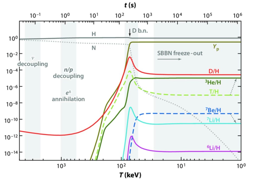
Though 1H and 4He are by far the most common products of BBN, there are traces of other isotopes that emerge from BBN:
The time evolution of the relative numbers of light element isotopes through BBN. As the universe expands, nuclear reactions “freeze-out” and establish primordial abundances for the indicated species. The precise outcome depends on the baryon density, Ωb. This plot illustrates a particular choice of Ωb; different Ωb result in observationally distinguishable abundances. (Figures like this are so ubiquitous in discussions of the early universe that I have not been able to identify the original citation for this particular version.)After hydrogen and helium, the next most common isotope to emerge from BBN is deuterium, 2H. It is the first thing made (one proton plus one neutron) but most of it gets processed into 4He, so after a brief peak, its abundance declines. How much it declines is very sensitive to Ωb: the higher the baryon density, the more deuterium gets gobbled up by helium before freeze-out. The following figure illustrates how the abundance of each isotope depends on Ωb:
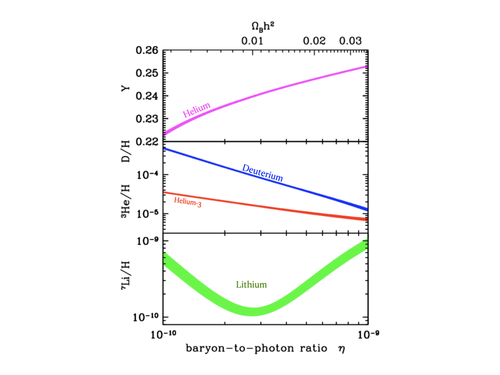
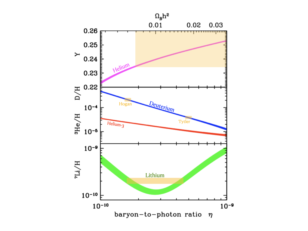
“Schramm diagram” adopted from Cyburt et al (2003) showing the abundance of 4He by mass fraction (top) and the number relative to hydrogen of deuterium (D = 2H), helium-3, and lithium as a function of the baryon-to-photon ratio. We measure the photon density in the CMB, so this translates directly to the baryon density$ Ωbh2 (top axis).If we can go out and measure the primordial abundances of these various isotopes, we can constrain the baryon density.
The Baryon Density
It works! Each isotope provides an independent estimate of Ωbh2, and they agree pretty well. This was the first and for a long time the only over-constrained quantity in cosmology. So while I am going to quibble about the exact value of Ωbh2, I don’t doubt that the basic picture is correct. There are too many details we have to get right in the complex nuclear reaction chains coupled to the decreasing temperature of a universe expanding at the rate required during radiation domination for this to be an accident. It is an exquisite success of the standard Hot Big Bang cosmology, albeit not one specific to LCDM.
Getting at primordial, rather than current, abundances is an interesting observational challenge too involved to go into much detail here. Suffice it to say that it can be done, albeit to varying degrees of satisfaction. We can then compare the measured abundances to the theoretical BBN abundance predictions to infer the baryon density.
The Schramm diagram with measured abundances (orange boxes) for the isotopes of the light elements. The thickness of the box illustrates the uncertainty: tiny for deuterium and large for 4He because of the large zoom on the axis scale. The lithium abundance could correspond to either low or high baryon density. 3He is omitted because its uncertainty is too large to provide a useful constraint.Deuterium is considered the best baryometer because its relic abundance is very sensitive to Ωbh2: a small change in baryon density corresponds to a large change in D/H. In contrast, 4He is a great confirmation of the basic picture – the primordial mass fraction has to come in very close to 1/4 – but the precise value is not very sensitive to Ωbh2. Most of the neutrons end up in helium no matter what, so it is hard to distinguish# a few more from a few less. (Note the huge zoom on the linear scale for 4He. If we plotted it logarithmically with decades of range as we do the other isotopes, it would be a nearly flat line.) Lithium is annoying for being double-valued right around the interesting baryon density so that the observed lithium abundance can correspond to two values of Ωbh2. This behavior stems from the trade off with 7Be which is produced at a higher rate but decays to 7Li after a few months. For this discussion the double-valued ambiguity of lithium doesn’t matter, as the problem is that the deuterium abundance indicates Ωbh2 that is even higher than the higher branch of lithium.
BBN pre-CMB
The diagrams above and below show the situation in the 1990s before CMB estimates became available. Consideration of all the available data in the review of Walker et al. led to the value Ωbh2 = 0.0125 ± 0.0025. This value** was so famous that it was Known. It formed the basis of my predictions for the CMB for both LCDM and no-CDM. This prediction hinged on BBN being correct, and that we understood the experimental bounds on the baryon density. A few years after Walker’s work, Copi et al. provided the estimate++ 0.009 < Ωbh2 < 0.02. Those were the extreme limits of the time, as illustrated by the green box below:
The baryon density as it was known before detailed observations of the acoustic power spectrum of the CMB. BBN was a mature subject before 1990; the massive reviews of Walker et al. and Copi et al. creak with the authority of a solved problem. The controversial tension at the time was between the high and low deuterium measurements from Hogan and Tytler, which were at the extreme ends of the ranges indicated by the bulk of the data in the reviews.Up until this point, the constraints on BBN had come mostly from helium observations in nearby galaxies and lithium measurements in metal poor stars. It was only just then becoming possible to obtain high quality spectra of sufficiently high redshift quasars to see weak deuterium lines associated with strongly damped primary hydrogen absorption in intergalactic gas along the line of sight. This is great: deuterium is the most sensitive baryometer, the redshifts were high enough to be early in the history of the universe close to primordial times, and the gas was in the middle of intergalactic nowhere so shouldn’t be altered by astrophysical processes. These are ideal conditions, at least in principle.
First results were binary. Craig Hogan obtained a high deuterium abundance, corresponding to a low baryon density. Really low. From my Walker et al.-informed confirmation bias, too low. It was a a brand new result, so promising but probably wrong. Then Tytler and his collaborators came up with the opposite result: low deuterium abundance corresponding to a high baryon density: Ωbh2 = 0.019 ± 0.001. That seemed pretty high at the time, but at least it was within the bound Ωbh2 < 0.02 set by Copi et al. There was a debate between these high/low deuterium camps that ended in a rare act of intellectual honesty by a cosmologist when Hogan&& conceded. We seemed to have settled on the high-end of the allowed range, just under Ωbh2 = 0.02.
Enter the CMB
CMB data started to be useful for constraining the baryon density in 2000 and improved rapidly. By that point, LCDM was already well-established, and I had published predictions for both LCDM and no-CDM. In the absences of cold dark matter, one expects a damping spectrum, with each peak lower than the one before it. For the narrow (factor of two) Known range of possible baryon densities, all the no-CDM models run together to essentially the same first-to-second peak ratio.
Peak locations measured by WMAP in 2003 (points) compared to the a priori (1999) predictions of LCDM (red tone lines) and no-CDM (blue tone lines). Models are normalized in amplitude around the first peak.Adding CDM into the mix adds a driver to the oscillations. This fights the baryonic damping: the CDM is like a parent pushing a swing while the baryons are the kid dragging his feet. This combination makes just about any pattern of peaks possible. Not all free parameters are made equal: the addition of a single free parameter, ΩCDM, makes it possible to fit any plausible pattern of peaks. Without it (no-CDM means ΩCDM = 0), only the damping spectrum is allowed.
For BBN as it was known at the time, the clear difference was in the relative amplitude$$ of the first and second peaks. As can be seen above, the prediction for no-CDM was correct and that for LCDM was not. So we were done, right?
Of course not. To the CMB community, the only thing that mattered was the fit to the CMB power spectrum, not some obscure prediction based on BBN. Whatever the fit said was True; too bad for BBN if it didn’t agree.
The way to fit the unexpectedly small## second peak was to crank up the baryon density. To do that, Tegmark & Zaldarriaga (2000) needed 0.022 < Ωbh2 < 0.040. That’s what the first blue point below. This was the first time that I heard it suggested that the baryon density could be so high.
The baryon density from deuterium (red triangles) before and after (dotted vertical line) estimates from the CMB (blue points). The horizontal dotted line is the pre-CMB upper limit of Copi et al.The astute reader will note that the CMB-fit 0.022 < Ωbh2 < 0.040 sits entirely outside the BBN bounds 0.009 < Ωbh2 < 0.02. So we’re done, right? Well, no – the community simply ignored the successful a priori prediction of the no-CDM scenario. That was certainly easier than wrestling with its implications, and no one seems to have paused to contemplate why the observed peak ratio came in exactly at the one unique value that it could obtain in the case of no-CDM.
For a few years, the attitude seemed to be that BBN was close but not quite right. As the CMB data improved, the baryon density came down, ultimately settling on Ωbh2 = 0.0224 ± 0.0001. Part of the reason for this decline from the high initial estimate is covariance. In this case, the tilt plays a role: the baryon density declined as ns = 1 → 0.965 ± 0.004. Getting the second peak amplitude right takes a combination of both.
Now we’re back in the ballpark, almost: Ωbh2 = 0.0224 is not ridiculously far above the BBN limit Ωbh2 < 0.02. Close enough for Spergel et al. (2003) to say “The remarkable agreement between the baryon density inferred from D/H values and our [WMAP] measurements is an important triumph for the basic big bang model.” This was certainly true given the size of the error bars on both deuterium and the CMB at the time. It also elides*** any mention of either helium or lithium or the fact that the new Known was not consistent with the previous Known. Ωbh2 = 0.0224 was always the ally; Ωbh2 = 0.0125 was always the enemy.
Note, however, that deuterium made a leap from below Ωbh2 = 0.02 to above 0.02 exactly when the CMB indicated that it should do so. They iterated to better agreement and pretty much stayed there. Hopefully that is the correct answer, but given the history of the field, I can’t help worrying about confirmation bias. I don’t know if that is what’s going on, but if it were, this convergence over time is what it would look like.
Lithium does not concur
Taking the deuterium results at face value, there really is excellent agreement with the LCDM fit to the CMB, so I have some sympathy for the desire to stop there. Deuterium is the best baryometer, after all. Helium is hard to get right at a precise enough level to provide a comparable constraint, and lithium, well, lithium is measured in stars. Stars are tiny, much smaller than galaxies, and we know those are too puny to simulate.
Spite & Spite (1982) [those are names, pronounced “speet”; we’re not talking about spiteful stars] discovered what is now known as the Spite plateau, a level of constant lithium abundance in metal poor stars, apparently indicative of the primordial lithium abundance. Lithium is a fragile nucleus; it can be destroyed in stellar interiors. It can also be formed as the fragmentation product of cosmic ray collisions with heavier nuclei. Both of these things go on in nature, making some people distrustful of any lithium abundance. However, the Spite plateau is a sort of safe zone where neither effect appears to dominate. The abundance of lithium observed there is indeed very much in the right ballpark to be a primordial abundance, so that’s the most obvious interpretation.
Lithium indicates a lowish baryon density. Modern estimates are in the same range as BBN of old; they have not varied systematically with time. There is no tension between lithium and pre-CMB deuterium, but it disagrees with LCDM fits to the CMB and with post-CMB deuterium. This tension is both persistent and statistically significant (Fields 2011 describes it as “4–5σ”).
The baryon density from lithium (yellow symbols) over time. Stars are measurements in groups of stars on the Spite plateau; the square represents the approximate value from the ISM of the SMC.I’ve seen many models that attempt to fix the lithium abundance, e.g., by invoking enhanced convective mixing via <<mumble mumble>> so that lithium on the surface of stars is subject to destruction deep in the stellar interior in a previously unexpected way. This isn’t exactly satisfactory – it should result in a mess, not a well-defined plateau – and other attempts I’ve seen to explain away the problem do so with at least as much contrivance. All of these models appeared after lithium became a problem; they’re clearly motivated by the assumption bias that the CMB is correct so the discrepancy is specific to lithium so there must be something weird about stars that explains it.
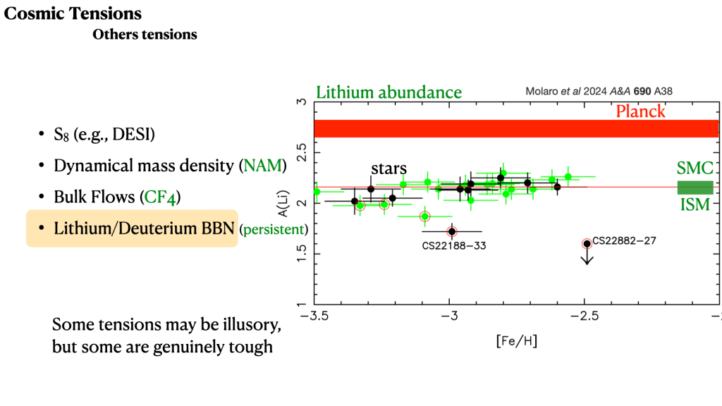
Another way to illustrate the tension is to use Ωbh2 from the Planck fit to predict what the primordial lithium abundance should be. The Planck-predicted band is clearly higher than and offset from the stars of the Spite plateau. There should be a plateau, sure, but it’s in the wrong place.
The lithium abundance in metal poor stars (points), the interstellar medium of the Small Magellanic Cloud (green band), and the primordial lithium abundance expected for the best-fit Planck LCDM. For reference, [Fe/H] = -3 means an iron abundance that is one one-thousandth that of the sun.An important recent observation is that a similar lithium abundance is obtained in the metal poor interstellar gas of the Small Magellanic Cloud. That would seem to obviate any explanation based on stellar physics.
The Schramm diagram with the Planck CMB-LCDM value added (vertical line). This agrees well with deuterium measurements made after CMB data became available, but not with those before, nor with the measured abundance of lithium. We can also illustrate the tension on the Schramm diagram. This version adds the best-fit CMB value and the modern deuterium abundance. These are indeed in excellent agreement, but they don’t intersect with lithium. The deuterium-lithium tension appears to be real, and comparable in significance to the H0 tension.
So what’s the answer?
I don’t know. The logical options are
- A systematic error in the primordial lithium abundance
- A systematic error in the primordial deuterium abundance
- Physics beyond standard BBN
I don’t like any of these solutions. The data for both lithium and deuterium are what they are. As astronomical observations, both are subject to the potential for systematic errors and/or physical effects that complicate their interpretation. I am also extremely reluctant to consider modifications to BBN. There are occasional suggestions to this effect, but it is a lot easier to break than it is to fix, especially for what is a fairly small disagreement in the absolute value of Ωbh2.
I have left the CMB off the list because it isn’t part of BBN: it’s constraint on the baryon density is real, but involves completely different physics. It also involves different assumptions, i.e., the LCDM model and all its invisible baggage, while BBN is just what happens to ordinary nucleons during radiation domination in the early universe. CMB fits are corroborative of deuterium only if we assume LCDM, which I am not inclined to accept: deuterium disagreed with the subsequent CMB data before it agreed. Whether that’s just progress or a sign of confirmation bias, I also don’t know. But I do know confirmation bias has bedeviled the history of cosmology, and as the H0 debate shows, we clearly have not outgrown it.
The appearance of confirmation bias is augmented by the response time of each measured elemental abundance. Deuterium is measured using high redshift quasars; the community that does that work is necessarily tightly coupled to cosmology. It’s response was practically instantaneous: as soon as the CMB suggested that the baryon density needed to be higher, conforming D/H measurements appeared. Indeed, I recall when that first high red triangle appeared in the literature, a colleague snarked to me “we can do that too!” In those days, those of us who had been paying attention were all shocked at how quickly Ωbh2 = 0.0125 ± 0.0025 was abandoned for literally double that value, ΩBh2 = 0.025 ± 0.001. That’s 4.6 sigma for those keeping score.
The primordial helium abundance is measured in nearby dwarf galaxies. That community is aware of cosmology, but not as strongly coupled to it. Estimates of the primordial helium abundance have drifted upwards over time, corresponding to higher implied baryon densities. It’s as if confirmation bias is driving things towards the same result, but on a timescale that depends on the sociological pressure of the CMB imperative.
Fig. 8 from
Steigman (2012) showing the history of primordial helium mass fraction (YP) determinations as a function of time. I am not accusing anyone of trying to obtain a particular result. Confirmation bias can be a lot more subtle than that. There is an entire field of study of it in psychology. We “humans actively sample evidence to support prior beliefs” – none of us are immune to it.
In this case, how we sample evidence depends on the field we’re active in. Lithium is measured in stars. One can have a productive career in stellar physics while entirely ignoring cosmology; it is the least likely to be perturbed by edicts from the CMB community. The inferred primordial lithium abundance has not budged over time.
What’s your confirmation bias?
I try not to succumb to confirmation bias, but I know that’s impossible. The best I can do is change my mind when confronted with new evidence. This is why I went from being sure that non-baryonic dark matter had to exist to taking seriously MOND as the theory that predicted what I observed.
I do try to look at things from all perspectives. Here, the CMB has been a roller coaster. Putting on an LCDM hat, the location of the first peak came in exactly where it was predicted: this was strong corroboration of a flat FLRW geometry. What does it mean in MOND? No idea – MOND doesn’t make a prediction about that. The amplitude of the second peak came in precisely as predicted for the case of no-CDM. This was corroboration of the ansatz inspired by MOND, and the strongest possible CMB-based hint that we might be barking up the wrong tree with LCDM.
As an exercise, I went back and maxed out the baryon density as it was known before the second peak was observed. We already thought we knew LCDM parameters well enough to do this. We couldn’t. The amplitude of the second peak came as a huge surprise to LCDM; everyone acknowledged that at the time (if pressed; many simply ignored it). Nowadays this is forgotten, or people have gaslit themselves into believing this was expected all along. It was not.
Fig. 45 from Famaey & McGaugh (2012):
WMAP data are shown with the a priori prediction of no-CDM (blue line) and the most favorable prediction that could have been made ahead of time for LCDM (red line).From the perspective of no-CDM, we don’t really care whether deuterium or lithium hits closer to the right baryon density. All plausible baryon densities predict essentially the same A1:2 amplitude ratio. Once we admit CDM as a possibility, then the second peak amplitude becomes very sensitive to the mix of CDM and baryons. From this perspective, the lithium-indicated baryon density is unacceptable. That’s why it is important to have a test that is independent of the CMB. Both deuterium and lithium provide that, but they disagree about the answer.
Once we broke BBN to fit the second peak in LCDM, we were admitting (if not to ourselves) that the a priori prediction of LCDM had failed. Everything after that is a fitting exercise. There are enough free parameters in LCDM to fit any plausible power spectrum. Cosmologists are fond of saying there are thousands of independent multipoles, but that overstates the case: it doesn’t matter how finely we sample the wave pattern, it matters what the wave pattern is. That is not as over-constrained as it is made to sound. LCDM is, nevertheless, an excellent fit to the CMB data; the test then is whether the parameters of this fit are consistent with independent measurements. It was until it wasn’t; that’s why we face all these tensions now.
Despite the success of the prediction of the second peak, no-CDM gets the third peak wrong. It does so in a way that is impossible to fix short of invoking new physics. We knew that had to happen at some level; empirically that level occurs at L = 600. After that, it becomes a fitting exercise, just as it is in LCDM – only now, one has to invent a new theory of gravity in which to make the fit. That seems like a lot to ask, so while it remained as a logical possibility, LCDM seemed the more plausible explanation for the CMB if not dynamical data. From this perspective, that A1:2 came out bang on the value predicted by no-CDM must just be one heck of a cosmic fluke. That’s easy to accept if you were unaware of the prediction or scornful of its motivation; less so if you were the one who made it.
Either way, the CMB is now beyond our ability to predict. It has become a fitting exercise, the chief issue being what paradigm in which to fit it. In LCDM, the fit follows easily enough; the question is whether the result agrees with other data: are these tensions mere hiccups in the great tradition of observational cosmology? Or are they real, demanding some new physics?
The widespread attitude among cosmologists is that it will be impossible to fit the CMB in any way other than LCDM. That is a comforting thought (it has to be CDM!) and for a long time seemed reasonable. However, it has been contradicted by the success of Skordis & Zlosnik (2021) using AeST, which can fit the CMB as well as LCDM.
CMB power spectrum observed by Planck fit by AeST (Skordis & Zlosnik 2021).AeST is a very important demonstration that one does not need dark matter to fit the CMB. One does need other fields+++, so now the reality of those have to be examined. Where this show stops, nobody knows.
I’ll close by noting that the uniqueness claimed by the LCDM fit to the CMB is a property more correctly attributed to MOND in galaxies. It is less obvious that this is true because it is always possible to fit a dark matter model to data once presented with the data. That’s not science, that’s fitting French curves. To succeed, a dark matter model must “look like” MOND. It obviously shouldn’t do that, so modelers refuse to go there, and we continue to spin our wheels and dig the rut of our field deeper.
Note added in proof, as it were: I’ve been meaning to write about this subject for a long time, but hadn’t, in part because I knew it would be long and arduous. Being deeply interested in the subject, I had to slap myself repeatedly to refrain from spending even more time updating the plots with publication date as an axis: nothing has changed, so that would serve only to feed my OCD. Even so, it has taken a long time to write, which I mention because I had completed the vast majority of this post before the IAU announced on May 15 that Cooke & Pettini have been awarded the Gruber prize for their precision deuterium abundance. This is excellent work (it is one of the deuterium points in the relevant plot above), and I’m glad to see this kind of hard, real-astronomy work recognized.
The award of a prize is a recognition of meritorious work but is not a guarantee that it is correct. So this does not alter any of the concerns that I express here, concerns that I’ve expressed for a long time. It does make my OCD feels obliged to comment at least a little on the relevant observations, which is itself considerably involved, but I will tack on some brief discussion below, after the footnotes.
*These methods were in agreement before they were in tension, e.g., Spergel et al. (2003) state: “The agreement between the HST Key Project value and our [WMAP CMB] value, h = 0.72 ±0.05, is striking, given that the two methods rely on different observables, different underlying physics, and different model assumptions.”
+Here I mean the abundance of the primary isotope of lithium, 7Li. There is a different problem involving the apparent overabundance of 6Li. I’m not talking about that here; I’m talking about the different baryon densities inferred separately from the abundances of D/H and 7Li/H.
&By convention, X, Y, and Z are the mass fractions of hydrogen, helium, and everything else. Since the universe starts from a primordial abundance of Xp = 3/4 and Yp = 1/4, and stars are seen to have approximately that composition plus a small sprinkling of everything else (for the sun, Z ≈ 0.02), and since iron lines are commonly measured in stars to trace Z, astronomers fell into the habit of calling Z the metallicity even though oxygen is the third most common element in the universe today (by both number and mass). Since everything in the periodic table that isn’t hydrogen and helium is a small fraction of the mass, all the heavier elements are often referred to collectively as metals despite the unintentional offense to chemistry.
$The factor of h2 appears because of the definition of the critical density ρc = (3H02)/(8πG): Ωb = ρb/ρc. The physics cares about the actual density ρb but Ωbh2 = 0.02 is a lot more convenient to write than ρb,now = 3.75 x 10⁻³¹ g/cm3.
#I’ve worked on helium myself, but was never able to do better than Yp = 0.25 ± 0.01. This corroborates the basic BBN picture, but does not suffice as a precise measure of the baryon density. To do that, one must obtain a result accurate to the third place of decimals, as discussed in the exquisite works of Kris Davidson, Bernie Pagel, Evan Skillman, and their collaborators. It’s hard to do for both observational reasons and because a wealth of subtle atomic physics effects come into play at that level of precision – helium has multiple lines; their parent population levels depend on the ionization mechanism, the plasma temperature, its density, and fluorescence effects as well as abundance.
**The value reported by Walker et al. was phrased as Ωbh502 = 0.05 ± 0.01, where h50 = H0/(50 km/s/Mpc); translating this to the more conventional h = H0/(100 km/s/Mpc) decreases these numbers by a factor of four and leads to the impression of more significant digits than were claimed. It is interesting to consider the psychological effect of this numerology. For example, the modern CMB best-fit value in this phrasing is Ωbh502 = 0.09, four sigma higher than the value Known from the combined assessment of the light isotope abundances. That seems like a tension – not just involving lithium, but the CMB vs. all of BBN. Amusingly, the higher baryon density needed to obtain a CMB fit assuming LCDM is close to the threshold where we might have gotten away without the dynamical need (Ωm > Ωb) for non-baryonic dark matter that motivated non-baryonic dark matter in the first place. (For further perspective at a critical juncture in the development of the field, see Peebles 1999).
The use of h50 itself is an example of the confirmation bias I’ve mentioned before as prevalent at the time, that Ωm = 1 and H0 = 50 km/s/Mpc. I would love to be able to do the experiment of sending the older cosmologists who are now certain of LCDM back in time to share the news with their younger selves who were then equally certain of SCDM. I suspect their younger selves would ask their older selves at what age they went insane, if they didn’t simply beat themselves up.
++Craig Copi is a colleague here at CWRU, so I’ve asked him about the history of this. He seemed almost apologetic, since the current “right” baryon density from the CMB now is higher than his upper limit, but that’s what the data said at the time. The CMB gives a more accurate value only once you assume LCDM, so perhaps BBN was correct in the first place.
&&Or succumbed to peer pressure, as that does happen. I didn’t witness it myself, so don’t know.
$$The absolute amplitude of the no-CDM model is too high in a transparent universe. Part of the prediction of MOND is that reionization happens early, causing the universe to be a tiny bit opaque. This combination came out just right for τ = 0.17, which was the original WMAP measurement. It also happens to be consistent with the EDGES cosmic dawn signal and the growing body of evidence from JWST.
##The second peak was unexpectedly small from the perspective of CDM; it was both natural and expected in no-CDM. At the time, it was computationally expensive to calculate power spectra, so people had pre-computed coarse grids within which to hunt for best fits. The range covered by the grids was informed by extant knowledge, of which BBN was only one element. From a dynamical perspective, Ωm > 0.2 was adopted as a hard limit that imposed an edge in the grids of the time. There was no possibility of finding no-CDM as the best fit because it had been excluded as a possibility from the start.
***Spergel et al. (2003) also say “the best-fit Ωbh2 value for our fits is relatively insensitive to cosmological model and dataset combination as it depends primarily on the ratio of the first to second peak heights (Page et al. 2003b)” which is of course the basis of the prediction I made using the baryon density as it was Known at the time. They make no attempt to test that prediction, nor do they cite it.
+++I’ve heard some people assert that this is dark matter by a different name, so is a success of the traditional dark matter picture rather than of modified gravity. That’s not at all correct. It’s just stage three in the list of reactions to surprising results identified by Louis Agassiz.
All of the figures below are from Cooke & Pettini (2018), which I employ here to briefly illustrate how D/H is measured. This is the level of detail I didn’t want to get into for either deuterium or helium or lithium, which are comparably involved.
First, here is a spectrum of the quasar they observe, Q1243+307. The quasar itself is not the object of interest here, though quasars are certainly interesting! Instead, we’re looking at the absorption lines along the line of sight; the quasar is being used as a spotlight to illuminate the gas between it and us.
Figure 1. Final combined and flux-calibrated spectrum of Q1243+307 (black histogram) shown with the corresponding error spectrum (blue histogram) and zero level (green dashed line). The red tick marks above the spectrum indicate the locations of the Lyman series absorption lines of the sub-DLA at redshift zabs = 2.52564. Note the exquisite signal-to-noise ratio (S/N) of the combined spectrum, which varies from S/N ≃ 80 near the Lyα absorption line of the sub-DLA (∼4300 Å) to S/N ≃ 25 at the Lyman limit of the sub-DLA, near 3215 Å in the observed frame.The big hump around 4330 Å is Lyman α emission from the quasar itself. Lyα is the n = 2 to 1 transition of hydrogen, Lyβ is the n = 3 to 1 transition, and so on. The rest frame wavelength of Lyα is far into the ultraviolet at 1216 Å; we see it redshifted to z = 2.558. The rest of the spectrum is continuum and emission lines from the quasar with absorption lines from stuff along the line of sight. Note that the red end of the spectrum at wavelengths longer than 4400 Å is mostly smooth with only the occasional absorption line. Blueward of 4300 Å, there is a huge jumble. This is not noise, this is the Lyα forest. Each of those lines is absorption from hydrogen in clouds at different distances, hence different redshifts, along the line of sight.
Most of the clouds in the Lyα forest are ephemeral. The cross section for Lyα is huge so It takes very little hydrogen to gobble it up. Most of these lines represent very low column densities of neutral hydrogen gas. Once in a while though, one encounters a higher column density cloud that has enough hydrogen to be completely opaque to Lyα. These are damped Lyα systems. In damped systems, one can often spot the higher order Lyman lines (these are marked in red in the figure). It also means that there is enough hydrogen present to have a shot at detecting the slightly shifted version of Lyα of deuterium. This is where the abundance ratio D/H is measured.
To measure D/H, one has not only to detect the lines, but also to model and subtract the continuum. This is a tricky business in the best of times, but here its importance is magnified by the huge difference between the primary Lyα line which is so strong that it is completely black and the deuterium Lyα line which is incredibly weak. A small error in the continuum placement will not matter to the measurement of the absorption by the primary line, but it could make a huge difference to that of the weak line. I won’t even venture to discuss the nonlinear difference between these limits due to the curve of growth.
Figure 2. Lyα profile of the absorption system at zabs = 2.52564 toward the quasar Q1243+307 (black histogram) overlaid with the best-fitting model profile (red line), continuum (long dashed blue line), and zero-level (short dashed green line). The top panels show the raw, extracted counts scaled to the maximum value of the best-fitting continuum model. The bottom panels show the continuum normalized flux spectrum. The label provided in the top left corner of every panel indicates the source of the data. The blue points below each spectrum show the normalized fit residuals, (data–model)/error, of all pixels used in the analysis, and the gray band represents a confidence interval of ±2σ. The S/N is comparable between the two data sets at this wavelength range, but it is markedly different near the high order Lyman series lines (see Figures 4 and 5). The red tick marks above the spectra in the bottom panels show the absorption components associated with the main gas cloud (Components 2, 3, 4, 5, 6, 8, and 10 in Table 2), while the blue tick marks indicate the fitted blends. Note that some blends are also detected in Lyβ–Lyε.
The above examples look pretty good. The authors make the necessary correction for the varying spectral sensitivity of the instrument, and take great care to simultaneously fit the emission of the quasar and the absorption. I don’t think they’ve done anything wrong; indeed, it looks like they did everything right – just as the people measuring lithium in stars have.
Still, as an experienced spectroscopist, there are some subtle details that make me queasy. There are two independent observations, which is awesome, and the data look almost exactly the same, a triumph of repeatability. The fitted models are nearly identical, but if you look closely, you can see the model cuts slightly differently along the left edge of the damped absorption around 4278 Å in the two versions of the spectrum, and again along the continuum towards the right edge.
These differences are small, so hopefully don’t matter. But what is the continuum, really? The model line goes through the data, because what else could one possibly do? But there is so much Lyα absorption, is that really continuum? Should the continuum perhaps trace the upper envelope of the data? A physical effect that I worry about is that weak Lyα is so ubiquitous, we never see the true continuum but rather continuum minus a tiny bit of extraordinarily weak (Gunn-Peterson) absorption. If the true continuum from the quasar is just a little higher, then the primary hydrogen absorption is unaffected but the weak deuterium absorption would go up a little. That means slightly higher D/H, which means lower Ωbh2, which is the direction in which the measurement would need to move to come into closer agreement with lithium.
Is the D/H measurement in error? I don’t know. I certainly hope not, and I see no reason to think it is. I do worry that it could be. The continuum level is one thing that could go wrong; there are others. My point is merely that we shouldn’t assume it has to be lithium that is in error.
An important check is whether the measured D/H ratio depends on metallicity or column density. It does not. There is no variation with metallicity as measured by the logarithmic oxygen abundance relative to solar (left panel below). Nor does it appear to depend on the amount of hydrogen in the absorbing cloud (right panel). In the early days of this kind of work there appeared to be a correlation, raising the specter of a systematic. That is not indicated here.
Figure 6. Our sample of seven high precision D/H measures (symbols with error bars); the green symbol represents the new measure that we report here. The weighted mean value of these seven measures is shown by the red dashed and dotted lines, which represent the 68% and 95% confidence levels, respectively. The left and right panels show the dependence of D/H on the oxygen abundance and neutral hydrogen column density, respectively. Assuming the Standard Model of cosmology and particle physics, the right vertical axis of each panel shows the conversion from D/H to the universal baryon density. This conversion uses the Marcucci et al. (2016) theoretical determination of the d(p,γ)3He cross-section. The dark and light shaded bands correspond to the 68% and 95% confidence bounds on the baryon density derived from the CMB (Planck Collaboration et al. 2016).
I’ll close by noting that Ωbh2 from this D/H measurement is indeed in very good agreement with the best-fit Planck CMB value. The question remains whether the physics assumed by that fit, baryons+non-baryonic cold dark mater+dark energy in a strictly FLRW cosmology, is the correct assumption to make.
#I