Lmst

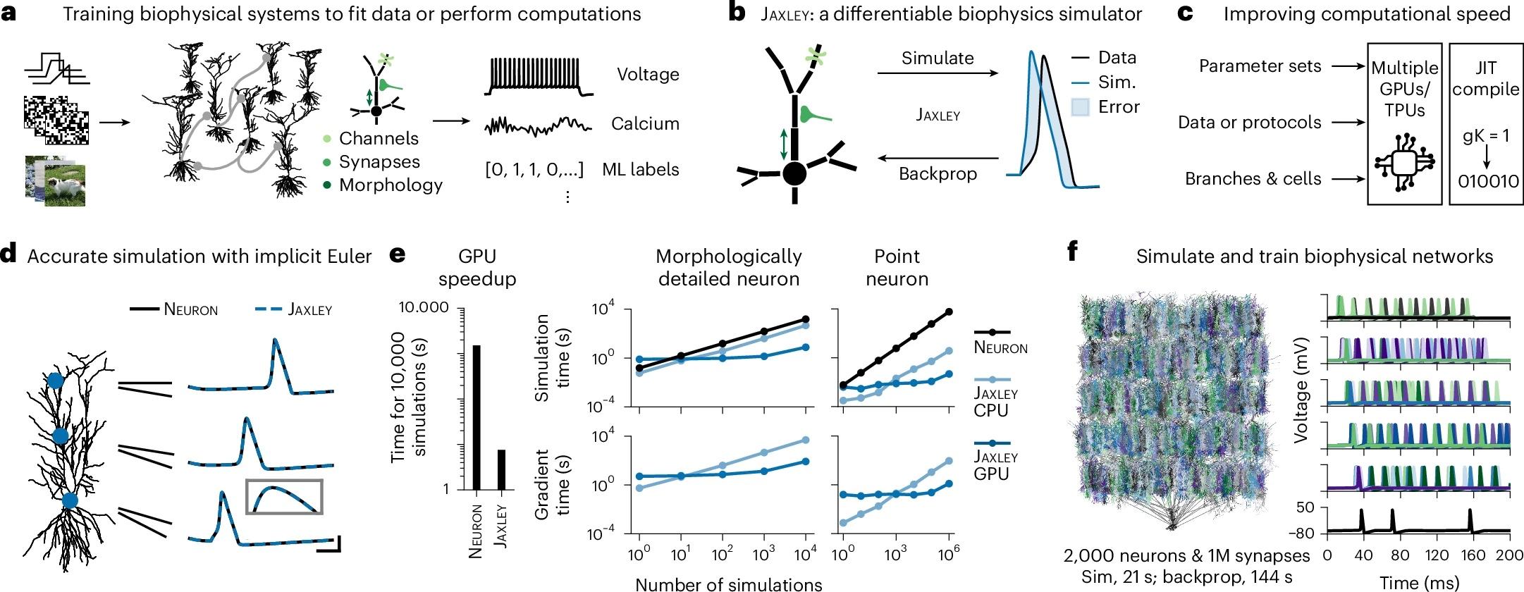
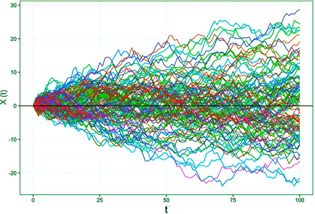
#NeuralDynamics is a central subfield of #ComputationalNeuroscience studying timedependent #NeuralActivity and its governing #mathematics. It examines how #NeuralStates evolve, how stable or unstable patterns arise, and how #learning reshapes them. Neural dynamics forms the backbone for how #neurons & #NeuralNetworks generate complex activity over time. This post gives a brief overview of the field & its historical milestones:

🌍https://www.fabriziomusacchio.com/blog/2026-02-04-neural_dynamics/

#CompNeuro #Neuroscience #DynamicalSystems

Phase plane (left) of an action potential generated by the FitzHugh–Nagumo model. Neural dynamics is largely concerned with understanding how such action potentials arise from the underlying biophysical and network dynamics. However, it also goes beyond and studies the dynamics of, e.g., neuronal populations, synaptic plasticity, and learning. In this post, we provide a definitional overview of the field of neural dynamics in order to situate it within the broader context of computational neuroscience and clarify some common misconceptions.

Spiking activity in a recurrent network of model neurons (Izhikevich model). Shown are the spike times of all neurons in a recurrent spiking neural network as a function of time. The network consists of 800 excitatory neurons with regular spiking (RS) dynamics and 200 inhibitory neurons with low-threshold spiking (LTS) dynamics, separated by the horizontal line. Each vertical mark corresponds to an action potential (spike) emitted by a single neuron. In the context of neural dynamics, this representation illustrates how single-neuron events, such as the action potentials described above, combine to form structured, time-dependent activity patterns at the network level. Such spiking rasters provide a direct link between microscopic neuronal dynamics and emerging population activity, which can later be analyzed in terms of collective states, low-dimensional structure, and neural manifolds.

Two complementary perspectives on population activity in neural dynamics. The figure contrasts a “circuit” perspective with a “neural manifold” perspective. In circuit models, neurons are organized in an abstract tuning space, where proximity reflects tuning similarity, and recurrent connectivity
W
i
j
together with external inputs generates time-dependent firing rates
r
i
(
t
)
(panels A–C). In the neural manifold view, the joint activity vector
r
(
t
)
∈
R
N
of a recorded population evolves along low-dimensional trajectories embedded in a high-dimensional space (panels D–F). This is illustrated by ring-like manifolds for head-direction representations and by rotational trajectories in motor cortex, both of which can often be captured by a small number of latent variables
κ
1
(
t
)
,
…
,
κ
D
(
t
)
with
D
≪
N
. In the context of our overview post here, I think, the figure highlights very well why neural dynamics naturally connects mechanistic network modeling with state-space descriptions of population activity. These are not competing accounts, but complementary levels of description that emphasize different aspects of the same underlying dynamical system. Source: Figure 1 from Pezon, Schmutz, Gerstner, Linking neural manifolds to circuit structure in recurrent networks, 2024, bioRxiv 2024.02.28.582565, DOI: 10.1101/2024.02.28.582565ꜛ (license: CC-BY-NC-ND 4.0)

🧠 New preprint by Shervani-Tabar, Brincat & @ekmiller on emergent #TravelingWaves in #RNN.

By aligning RNN dynamics to an empirically measured #NeuralManifold, they show that task-relevant TW can emerge through #learning, w/o hard-coding wave dynamics or connectivity. The cool thing here is that the waves are not imposed or engineered, but emerge naturally from learning under #BiologicallyPlausible constraints:

🌍 https://doi.org/10.64898/2026.01.08.698281

#Neuroscience #CompNeuro #NeuralDynamics #WorkingMemory

Figure 1: Latent manifold alignment enables persistent traveling waves in the network during working memory delay

🧠 New preprint by Behrad et al. introducing #fastDSA, a much faster way to compare neural systems at the level of their dynamics, not just geometry or task performance.

What’s cool here: similarity is defined by shared #VectorFields, i.e. by the computational mechanism itself. This provides the first tool for mechanistic comparison of neural computations (to my knowledge).

🌍 https://arxiv.org/abs/2511.22828
💻 https://github.com/CMC-lab/fastDSA

#Neuroscience #CompNeuro #NeuralDynamics #Manifolds #DynamicalSystems

Figure 1. Schematic overview of methods for estimating dynamic (dis)similarity: DSA, family of fastDSA methods, and kwDSA.

Figure 2. Demonstration of automatic rank reduction with SVHT:

🧠 New preprint by Lee et al.: Fast dendritic excitations primarily mediate #backpropagation in #CA1 pyramidal #neurons during #behavior

Using kHz #VoltageImaging across the full #dendritic tree, they show that fast dendritic spikes are usually driven by somatic #bAPs, not independently initiated. #bAP propagation into apical dendrites is contin. modulated by pre-spike dendritic voltage & can trigger slower plateau potentials linked to complex spikes.

🌍https://doi.org/10.64898/2026.01.03.696606

#NeuralDynamics

Figure 1. Dendritic voltage imaging of CA1 pyramidal neurons in vivo.
(A) Genetic constructs to express Optopatch-V, comprising a voltage indicator, Voltron2-
JF608, and optogenetic actuator, CheRiff. Lucy-Rho (LR) motifs were used to improve
dendritic trafficking of both optogenetic tools.
(B) Microprism (1.5 × 1.5 × 2.5 mm) implanted along the anterior-posterior axis provides a
side-on view of CA1 pyramidal neurons.
(C) The optical setup contained two digital micromirror devices (DMDs) for targeted
illumination and targeted optogenetic stimulation.

(D) Maximum z-projection of a spinning disk confocal image of a CA1 pyramidal neuron
imaged through a prism in an anesthetized mouse, imaged via Voltron2-JF608
fluorescence.
(E) Voltage traces from dendritic branches of the neuron shown in (D) during wide-area
optogenetic stimulation in an anesthetized mouse.
(F) Zoomed-in trace of the dotted region in (E). Bottom: corresponding voltage kymograph
along the basal-apical axis (arrow line in (D)) showing bAP propagation along the apical
dendrite.
(G) Spike-triggered average (n = 94 spikes) of the spike waveform. Left: color-coded from
basal to apical dendrites. Right: kymograph along the basal-apical axis showing spike
initiation at the soma, and propagation delays, and attenuation along the dendrites.

🧠 New paper by Deistler et al: #JAXLEY: differentiable #simulation for large-scale training of detailed #biophysical #models of #NeuralDynamics.

They present a #differentiable #GPU accelerated #simulator that trains #morphologically detailed biophysical #neuron models with #GradientDescent. JAXLEY fits intracellular #voltage and #calcium data, scales to 1000s of compartments, trains biophys. #RNNs on #WorkingMemory tasks & even solves #MNIST.

🌍 https://doi.org/10.1038/s41592-025-02895-w

#Neuroscience #CompNeuro

Fig. 1: Differentiable simulation enables training biophysical neuron models.

🧠 New #preprint by Komi et al. (2025): Neural #manifolds that orchestrate walking and stopping. Using #Neuropixels recordings from the lumbar spinal cord of freely walking rats, they show that #locomotion arises from rotational #PopulationDynamics within a low-dimensional limit-cycle #manifold. When walking stops, the dynamics collapse into a postural manifold of stable fixed points, each encoding a distinct pose.

🌍 https://doi.org/10.1101/2025.11.08.687367

#CompNeuro #NeuralDynamics #Attractor #Neuroscience

Fig. 1. Model of spinal motor network and the walk-to-stop transitions: Bifurcation from limit cycle to a
fixed point attractor.

🧠 New preprint by Codol et al. (2025): Brain-like #NeuralDynamics for #behavioral control develop through #ReinforcementLearning. They show that only #RL, not #SupervisedLearning, yields neural activity geometries & dynamics matching monkey #MotorCortex recordings. RL-trained #RNNs operate at the edge of #chaos, reproduce adaptive reorganization under #visuomotor rotation, and require realistic limb #biomechanics to achieve brain-like control.

🌍 https://doi.org/10.1101/2024.10.04.616712

#CompNeuro #Neuroscience

Fig. 2: Neural networks trained with RL or SL achieved high performance in controlling the effector .

🧠 New paper by Clark et al. (2025) shows that the #dimensionality of #PopulationActivity in #RNN can be explained by just two #connectivity parameters: effective #CouplingStrength and effective #rank. Uses networks with rapidly decaying singular value spectra and structured overlaps between left and right singular vectors. Could be useful for interpreting large scale population recordings and connectome data I guess:

🌍 https://doi.org/10.1103/2jt7-c8cq

#CompNeuro #NeuralDynamics #Connectome

Fig. 2.
Schematic of the random-mode model. Upper: couplings
J
are generated as a sum of outer products,
ℓ
a
r
a
T
, with component strengths
D
a
. Lower: the two-point function
C
⋆
ϕ
(
τ
)
and four-point function
Ψ
⋆
ϕ
(
τ
)
are calculated in terms of the statistics of
D
a
. The two-point function depends only on the effective gain
g
eff
, while the four-point function depends on both
g
eff
and
PR
D
, the effective dimension of the connectivity determined by the
D
a
distribution.

🧠 New preprint by Kashefi et al. (2025): High-density #Neuropixels recordings in monkeys reveal compositional #NeuralDynamics in #MotorCortex. A posture subspace anchors fixed points, rotational dynamics link them to generate movement, and a uniform shift tracks trial state. Recurrent models show this geometry emerges only when controlling a full arm, suggesting posture-dependent control as a core principle:

🌍 https://www.biorxiv.org/content/10.1101/2025.09.04.674069v1

#Neuroscience #MotorControl #CompNeuro

Figure 3| Rotational dynamics
connect posture-specific fixed points
during reaching.
A) Hand trajectories and speed profiles
for six trial types involving reaches
between three diagonal targets. Colors
indicate reach direction.
B) Left: M1 Neural trajectories for each
reach condition. Dotted traces
represent center-out reaches. Each
trace begins at a black marker indicating
the start location, shaped as a plus,
square, or circle corresponding to trials
that began from the plus, square, or
circle target, respectively. Traces are
colored by reach direction, and arrows
indicate the go cue. Each trace ends in a
colored marker (plus, square, or circle)
representing the end target location.
Right: Same as left, but for the trial
types shown in panel A (right).
C) Neural trajectories projected onto
the top three principal components
(PCs) from a PCA fit across all 20
conditions. Each trace represents one
reach condition, colored by reach
direction. As in panel B, black markers
indicate start locations and colored
markers indicate end locations.
D–F) Same as panels A–C, but for
Monkey P

🖥 @fzj just inaugurated #JUPITER, #Europe’s first #exascale #supercomputer. Must be fun to run models on that thing. Finally scaling #NeuralDynamics 🧪🧮 by population size and complexity without melting your workstation 🤪

🌍 https://www.fz-juelich.de/en/jupiter

📚 New preprint by Song et al.: Geometry of #NeuralDynamics along the #cortical #attractor landscape reflects changes in attention. They show that while attractor positions are determined by cortical organization, the geometry of neural dynamics on the landscape changes systematically with attentional states and contexts.

🌍 https://www.biorxiv.org/content/10.1101/2025.08.08.669432v1

#Neuroscience #Attention #fMRI #CompNeuro

Figure 1. Schematics of the geometry of neural dynamics on the attractor landscape. A state space is defined where each dimension represents the activity of a brain region spanning the cortex. The hills and valleys represent the attractor landscape with valleys indicating the attractors. Each attractor corresponds to a recurring brain state that is identified from large-scale patterns of regional activity and interaction. The circles represent the neural activity at a specific moment. The trajectory of neural activity (indicated with black arrow) is largely determined by the landscape but can also be affected by external perturbations. For example, the red circle is more likely to fall toward the attractor based on the intrinsic landscape but may
move away from the attractor when perturbed by external forces, such as stimuli, task demands, or
behaviors. The speed and direction of the movement on this landscape defines the geometry of neural dynamics. Example brain state figures are adapted from Song et al. (2023).

🧠Could quantum noise shape the way we understand neural behavior?

This study explores how quantum noise influences the FitzHugh-Nagumo equations, a fundamental model for describing neuronal activity and excitable systems.

🔗 The FitzHugh-Nagumo equations and quantum noise. Computational and Structural Biotech Journal, DOI: https://doi.org/10.1016/j.csbj.2025.02.023

📚 CSBJ Quantum Biology & Biophotonics: https://www.csbj.org/qbio

#QuantumBiology #Brain #AI #QuantumNeuroscience #NeuralDynamics #QuantumPhysics

The FitzHugh-Nagumo equations and quantum noise. Computational and Structural Biotechnology Journal, DOI: https://doi.org/10.1016/j.csbj.2025.02.023

Preserved neural dynamics across animals performing similar behaviour | Nature: https://www.nature.com/articles/s41586-023-06714-0

#Neuroscience #NeuralDynamics #MotorCortex

An important step in #ComputationalNeuroscience 🧠💻 was the development of the #HodgkinHuxley model, for which Hodgkin and Huxley received the #NobelPrize in 1963. The model describes the dynamics of the #MembranePotential of a #neuron 🔬 by incorporating biophysiological properties. See here how it is derived, along with a simple implementation in #Python:

🌍 https://www.fabriziomusacchio.com/blog/2024-04-21-hodgkin_huxley_model/

Feel free to share and to experiment with the code.

#CompNeuro #PythonTutorial #NeuralDynamics #DynamicalSystem

A set of membrane potentials modelled by the Hodgkin-Huxley model. Different currents were used to model the membrane potential.

Check out this #NeurIPS2023 paper by Dinc et al. (2023) who introduce #CORNN, convex #optimization of recurrent neural networks for rapid inference of #NeuralDynamics:

🌍 https://arxiv.org/abs/2311.10200

#CompNeuro #Neuroscience #RNN

Figure 1: Using data-constrained recurrent neural networks for the interpretation and manipulationofbraindynamicswithinapotentialexperimentalpipeline. Thisapproachcenters around online modeling of network dynamics, which can enhance hypothesis testing at the single-cell level and support advancements in brain-machine interface research. The training process is motivated by three objectives: (i) predicting the patterns of neural populations, (ii) revealing inherent attractor structures, and (iii) formulating optimal control strategies for subsequent interventions.

Eviatar Yemini will talk Todayw about "A Tale of Two Sexes: The #NeuralDynamics of #Dimorphic #Behavior"

⏰ September 18, 2023, 11 am CET
📍 #iBehave seminar series, #MPI Lecture Hall (at #Caesar), Ludwig-Erhard-Allee 2, 53175 Bonn / online
🌍 https://ibehave.nrw/news-and-events/ibehave-seminar-series-talk-by-prof-dr-eviatar-yemini/

#neuroscience #CElegans #behaviourscience

#NeuralDynamics

Client Info