Lmst

#crustal

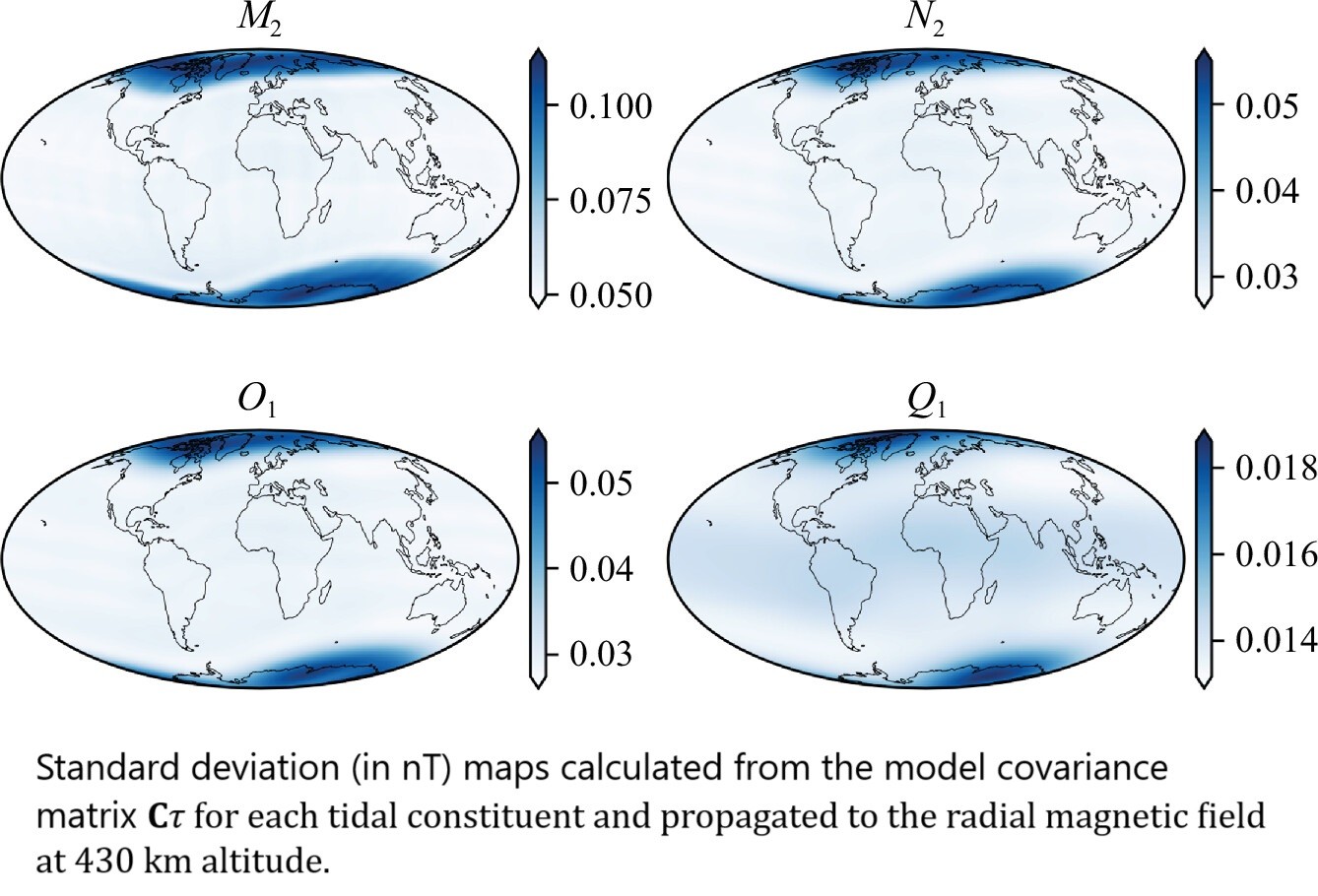
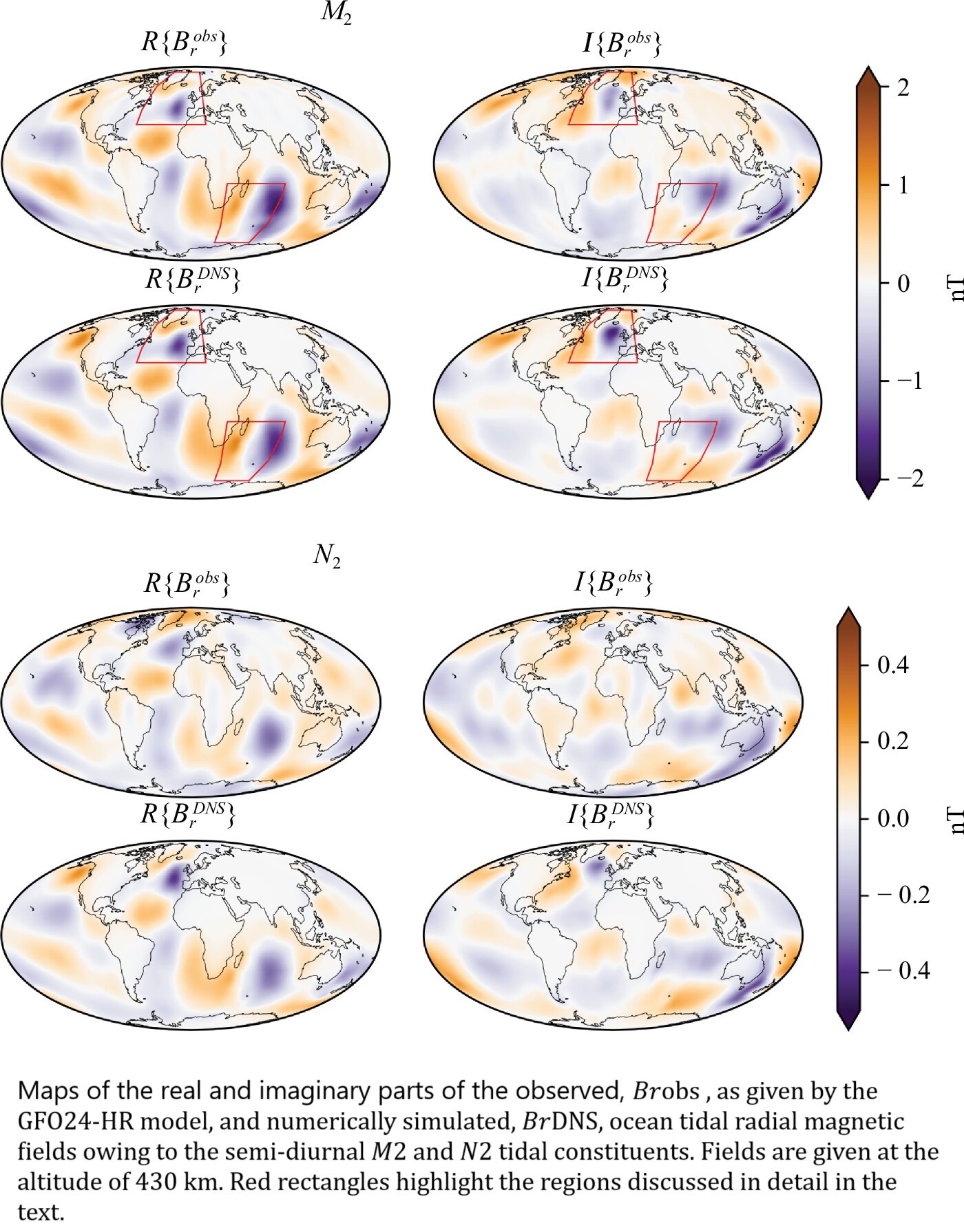
[SWARM] Satellites Detect Hidden Magnetic Signals In Earth's Oceans
--
https://www.earth.com/news/satellites-detect-hidden-magnetic-signals-in-earths-oceans/ <-- shared technical article
--
https://doi.org/10.1098/rsta.2024.0078 <-- shared paper
--
https://www.esa.int/Applications/Observing_the_Earth/FutureEO/Swarm <-- shared ESA SWARM home page
--
#GIS #spatial #mapping #remotesensing #ESA #SWARM #earthobservation #geomagnetism #magnetism #earth #global #magnetic #ocean #marine #tide #tidal #tidalinfluence #monitoring #spatialanalysis #spatiotemporal #model #modeling #magma #crustal #geology #structuralgeology #crust #plate #geophysics #geophysical #vulcanism

global maps - Standard deviation (in nT) maps calculated from the model covariance matrix 𝐂𝜏 for each tidal constituent and propagated to the radial magnetic field at 430 km altitude.

schematic - ocean, crust, magnetic field lines

global maps - Maps of the real and imaginary parts of the observed, 𝐵𝑟obs, as given by the GFO24-HR model, and numerically simulated, 𝐵𝑟DNS, ocean tidal radial magnetic fields owing to the semi-diurnal 𝑀2 and 𝑁2 tidal constituents. Fields are given at the altitude of 430 km. Red rectangles highlight the regions discussed in detail in the text.

global maps - Same as similar other figure, but for the diurnal 𝑂1 and 𝑄1 tidal constituents.

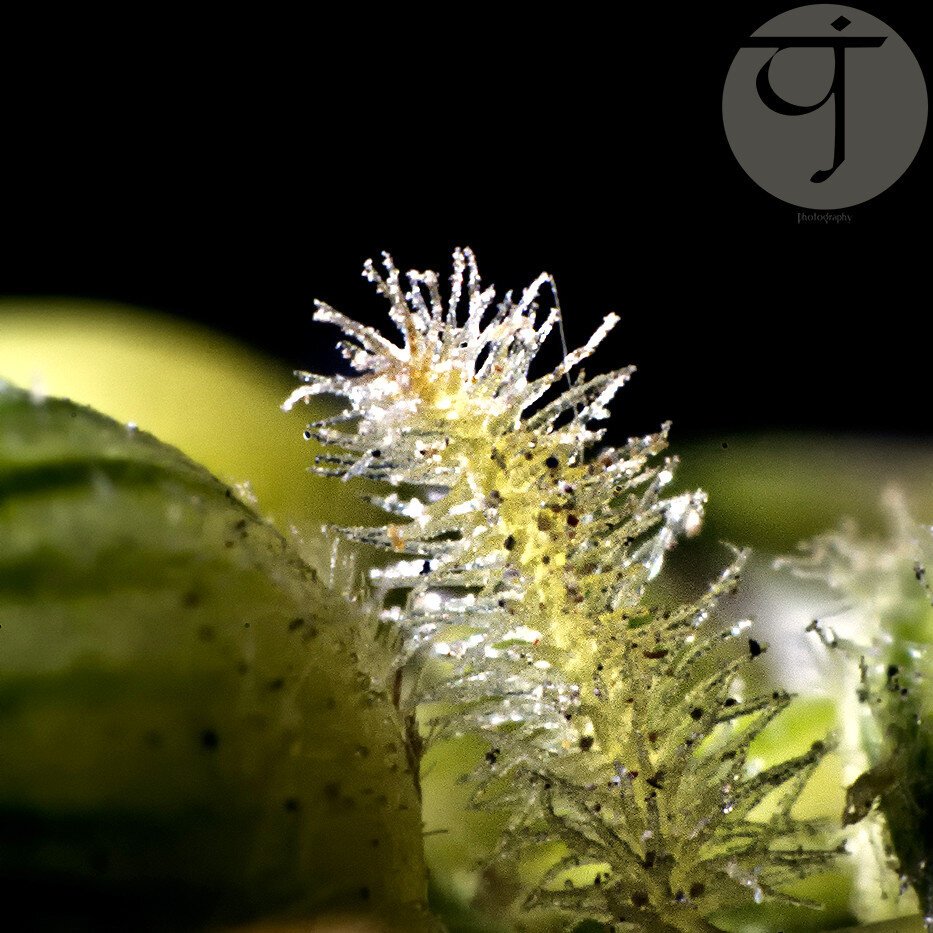
Crystalline 2;

I think this is the end of this series, but probably the fun just began! I'm currently working on some shots I've taken for some parts of this plant through the microscope. It is a struggle already, but hopefully I'll get to something. Lot of focus stacking needed here and, well, I don't have the proper tools, so, there will be lot of mishaps and cropping!

#nature #natural #macro #extrememacro #macrophotography #plants #crustal #crystalline #goodmorning

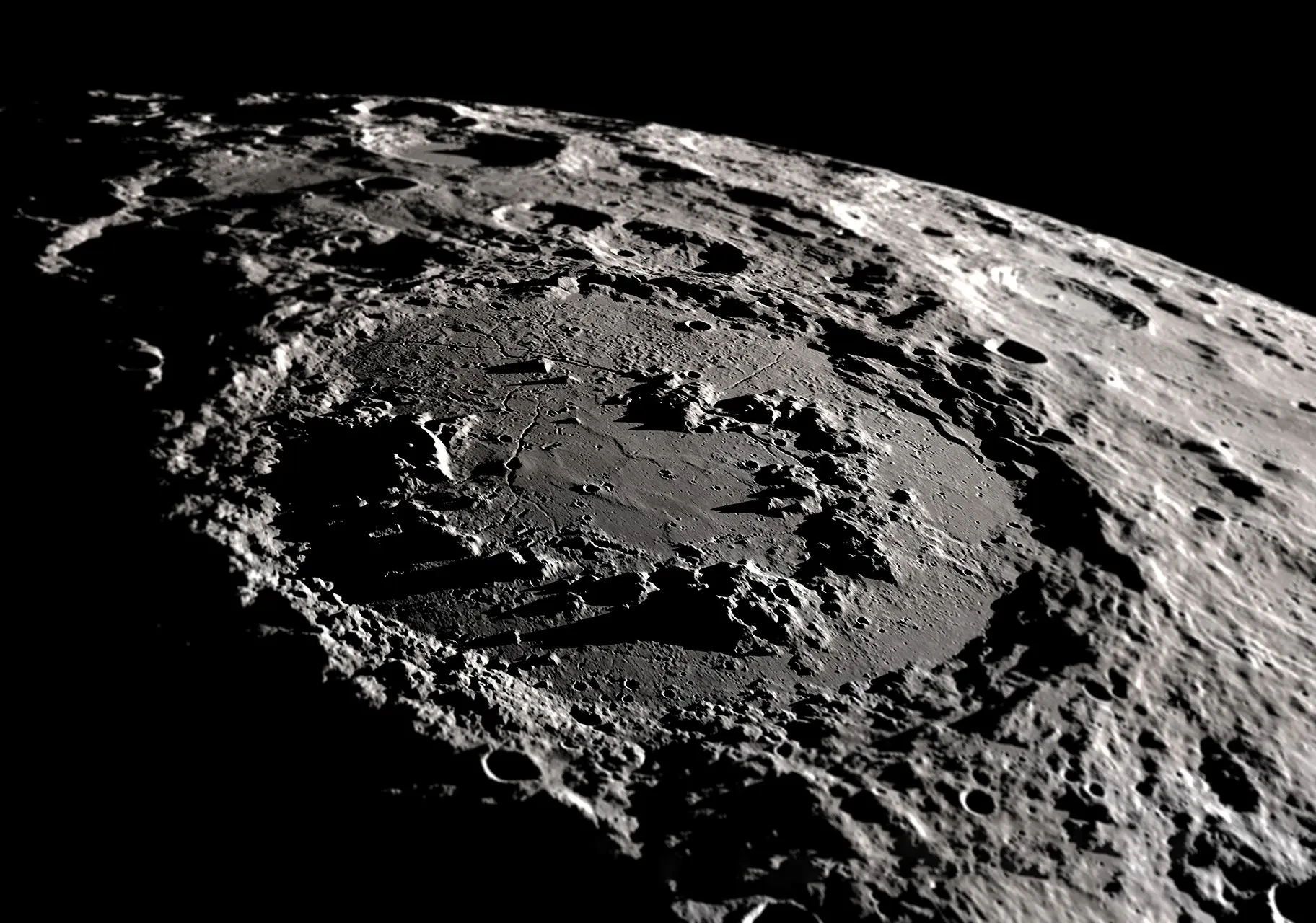
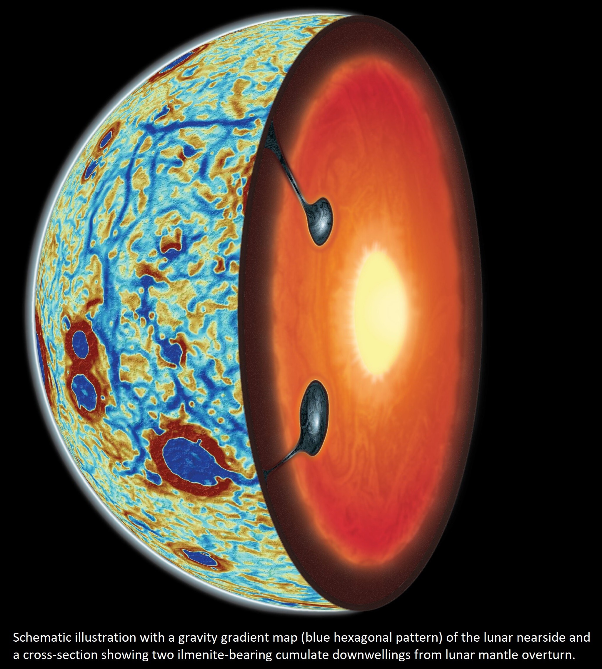
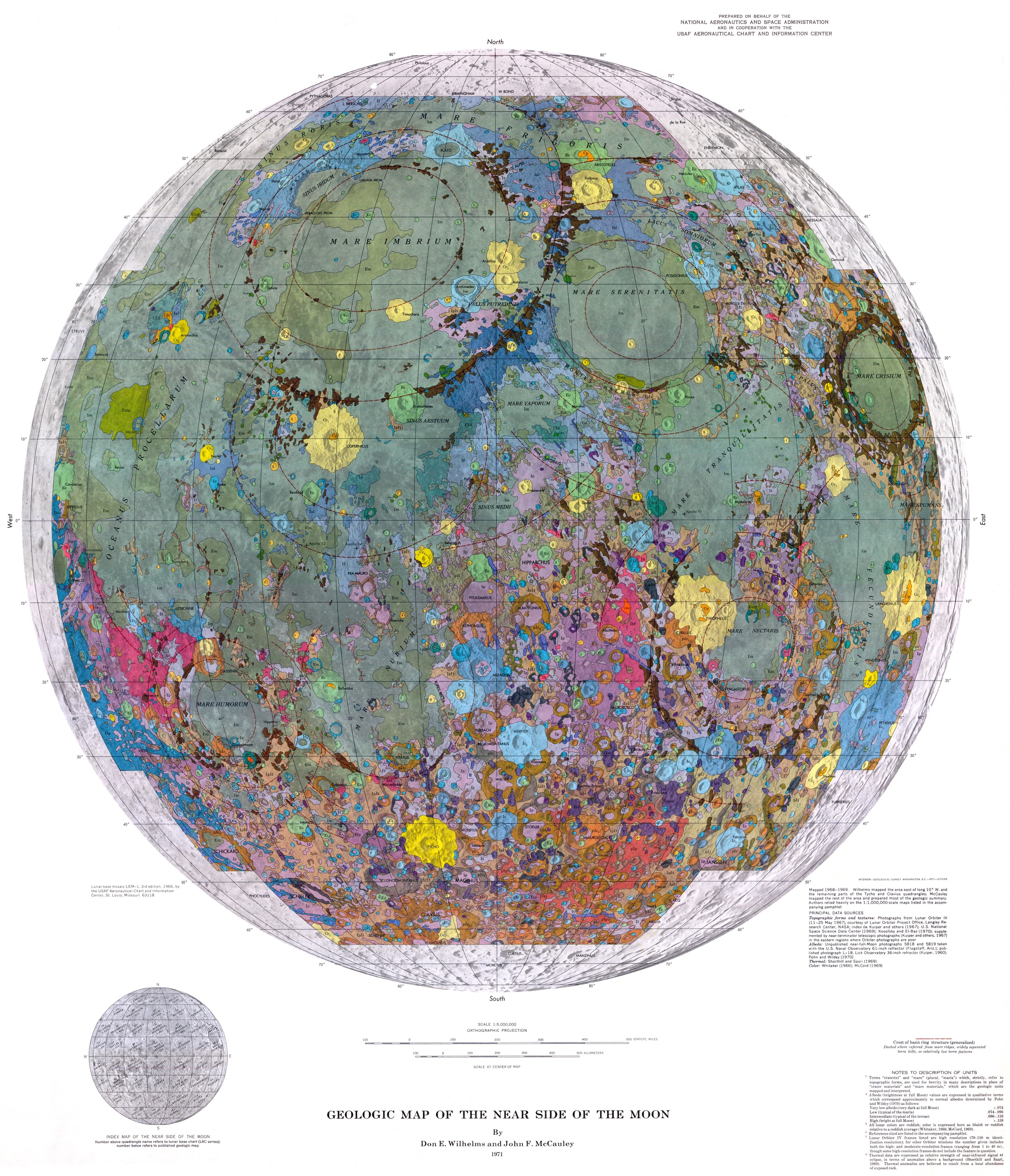
Scientists Solve A Long-Standing Mystery Surrounding The Moon's 'Lopsided' Geology
--
https://phys.org/news/2024-04-scientists-mystery-moon-lopsided-geology.html <-- shared technical article
--
https://doi.org/10.1038/s41561-024-01408-2 <-- shared paper
--
#GIS #spatial #mapping #modeling #model #research #moon #extraterrestrial #geology #remotesensing #lunar #structuralgeology #planetarygeology #lunarlandings #apollo #rocksamples #lava #crustal #mantle #solarsystem #magma #gravity #geodynamic #gravityanomalies #spatialanalysis #spatiotemporal #3dmodeling

Global maps of lunar topography, surface abundance of TiO2 and Bouguer gravity gradient [moon]

view of part of the moon's surface

Schematic illustration with a gravity gradient map (blue hexagonal pattern) of the lunar nearside and a cross-section showing two ilmenite-bearing cumulate downwellings from lunar mantle overturn.

USGS map (partial) - geologic map of the near side of the moon

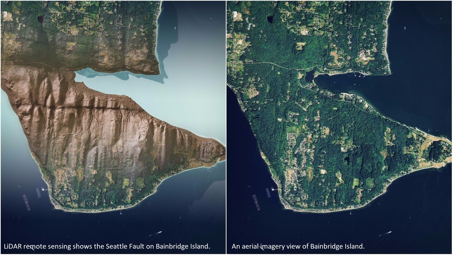
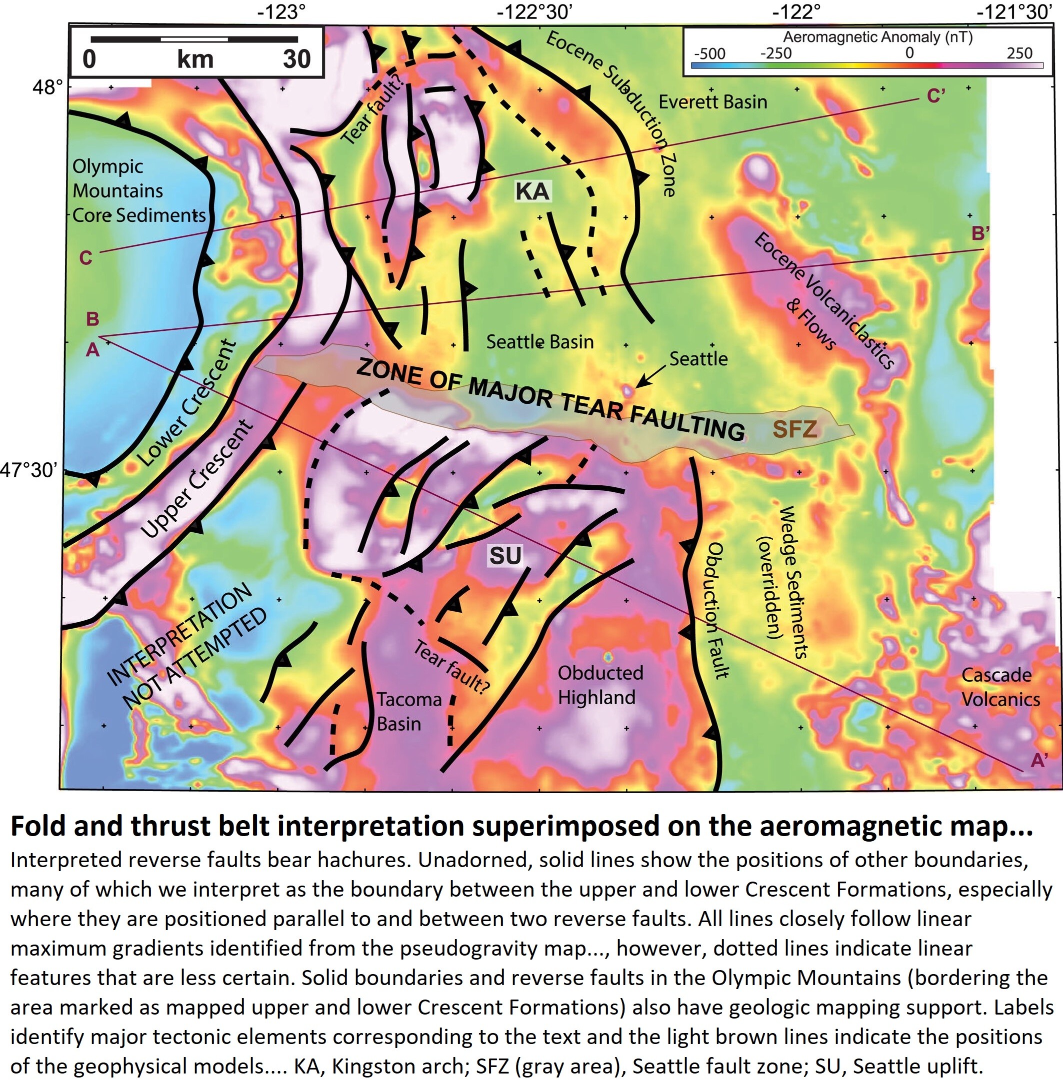
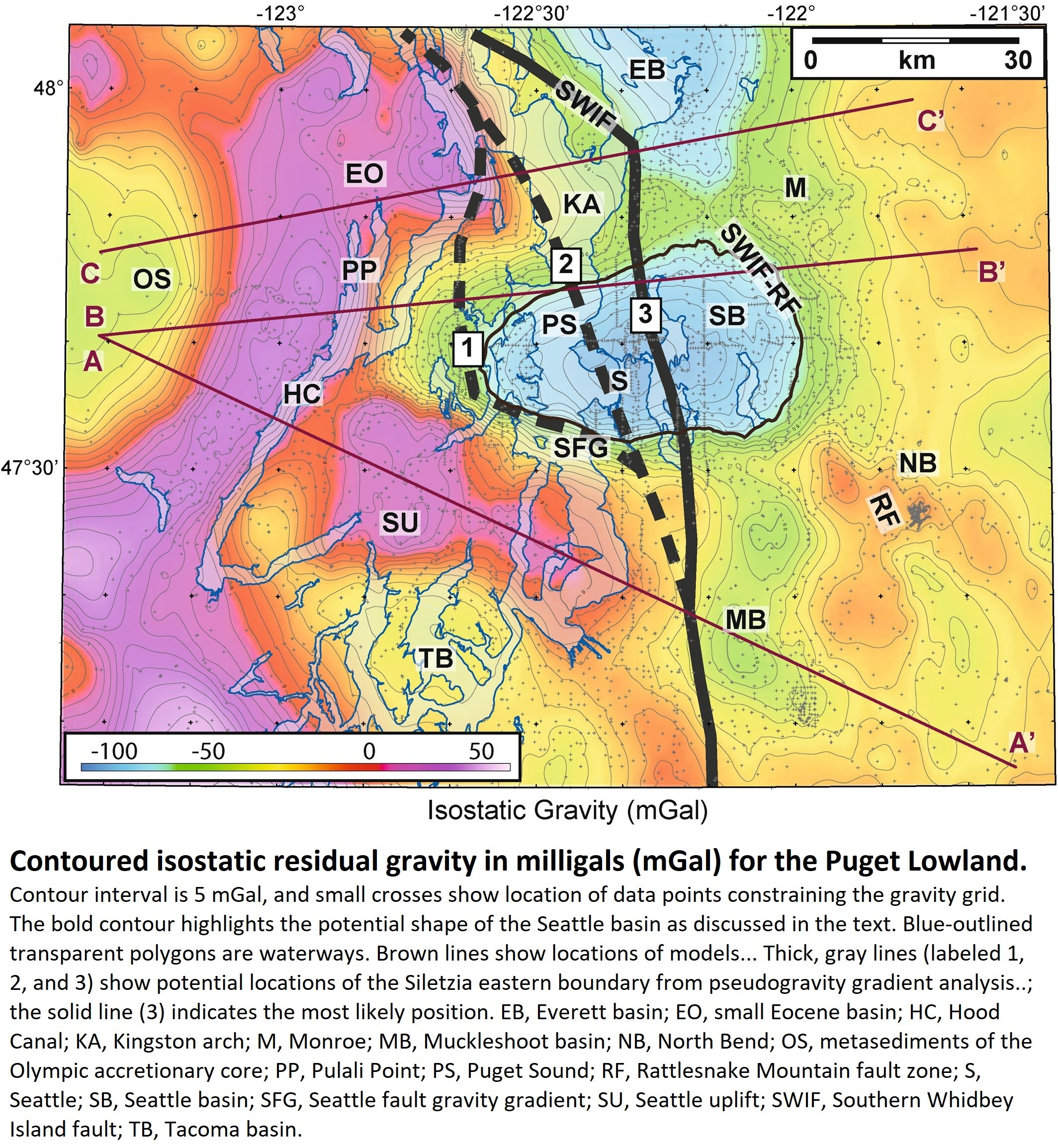
Deep Structure of Siletzia in the Puget Lowland - Imaging an Obducted Plateau and Accretionary Thrust Belt With Potential Fields
--
https://doi.org/10.1029/2022TC007720 <--shared paper
--
[I used to live, work as an engineering geologist and scuba dive in Puget Sound & beyond – including on the expressions of the Seattle Fault…]
#GIS #spatial #mapping #engineeringgeology #Seattle #pugetsound #washingtonstate #fault #faulting #earthquake #tsunami #structuralgeology #PNW #plateboundary #crustal #tectonics #cascadia #forearc #siletzia #seismic #seismichazard #geologichazard #risk #hazard #glacial #sediments #pugetlowland #model #modeling #remotesensing #magnetic #aeromagnetism #gravity #folding #thrust #geologicmapping #geology #seismology #accretionary #obduction #spatialanalysis #spatiotemporal #seattlefault #earthquakehazard #earthquakeengineering

imagery / photos - aerial - remotesensing sensing - LiDAR - the expression of the Seattle Fault on southern Bainbridge Island

map and model - Fold and thrust belt interpretation superimposed on the aeromagnetic map shown in Figure 4. Interpreted reverse faults bear hachures. Unadorned, solid lines show the positions of other boundaries, many of which we interpret as the boundary between the upper and lower Crescent Formations, especially where they are positioned parallel to and between two reverse faults. All lines closely follow linear maximum gradients identified from the pseudogravity map (Figure 5), however, dotted lines indicate linear features that are less certain. Solid boundaries and reverse faults in the Olympic Mountains (bordering the area marked as mapped upper and lower Crescent Formations) also have geologic mapping support. Labels identify major tectonic elements corresponding to the text and the light brown lines indicate the positions of the geophysical models in Figures 8-10. KA, Kingston arch; SFZ (gray area), Seattle fault zone; SU, Seattle uplift.

graphic / map - hillshade and annotations showing the Seattle Fault Zone, Puget Sound

map and model - Contoured isostatic residual gravity in milligals (mGal) for the Puget Lowland. Contour interval is 5 mGal, and small crosses show location of data points constraining the gravity grid. The bold contour highlights the potential shape of the Seattle basin as discussed in the text. Blue-outlined transparent polygons are waterways. Brown lines show locations of models in Figures 8-10 (A–A′, B–B′, and C–C′, respectively). Thick, gray lines (labeled 1, 2, and 3) show potential locations of the Siletzia eastern boundary from pseudogravity gradient analysis shown in Figure 5 and discussed in the text; the solid line (3) indicates the most likely position. EB, Everett basin; EO, small Eocene basin; HC, Hood Canal; KA, Kingston arch; M, Monroe; MB, Muckleshoot basin; NB, North Bend; OS, metasediments of the Olympic accretionary core; PP, Pulali Point; PS, Puget Sound; RF, Rattlesnake Mountain fault zone; S, Seattle; SB, Seattle basin; SFG, Seattle fault gravity gradient; SU, Seattle uplift; SWIF, Southern Whidbey Island fault; TB, Tacoma basin.

How The Indian Ocean Geoid Low Was Formed
--
https://doi.org/10.1029/2022GL102694 <-- shared paper
--
#GIS #spatial #mapping #remotesensing #gravity #geoid #geodesy #IndianOcean #formation #IOGL #model #modeling #geophysics #structuralgeology #crustal #mantle #convection #Tethyan #sea #ocean #subsidence #anomaly #spatialanalysis #spatiotemporal #tomography #density #rock #geology #tectonics #platetectonics

Client Info

Server: https://mastodon.social

Version: 2025.04

Repository: https://github.com/cyevgeniy/lmst